Summary Analysed coins Analysis

Summary

In the Coin Catalogue, the Nagidos staters are divided into three groups. It appears that the weight standard used for coins of Group 2 was approximately 0.11 g heavier than the weight standard used for Group 1, with the lowest weight standard being used for coins of Group 3 (approximately 0.57 g less than Group 1). The exceptions, however, are Type 1.5e in Group 1 and Type 2.8 in Group 2, whose weights correspond to Group 3. These two types were thus probably struck later than the other types of Groups 1 and 2.

Analysed coins

Coin catalogue section:	Nagidos
Coin corpus datasets:	Nagidos, Staters – Group 1, Nagidos, Staters – Group 2, Nagidos, Staters – Group 3

The numbers of analysed coins are given in Table 1. Coins whose weight is unknown or unreliable, or that are excessively corroded or damaged, are excluded from the analysis.

Corpus	Number of coins as of 1 November 2025
	Total	Excluded	Analysed
Nagidos, Staters – Group 1	143	1	142
Nagidos, Staters – Group 2	249	1	248
Nagidos, Staters – Group 3	202	7	195

Table 1: Numbers of analysed coins

Analysis

Box plots1 of individual coin types and basic descriptive statistics are presented in Figure 1 and Table 2 (Std. Dev. denotes the standard deviation and IQR the interquartile range), respectively. Type 1.5 is divided into variants 1.5a–d and 1.5e because specimens of variant 1.5e differ significantly in weight from the other variants of this type and, in addition to the differently placed ethnic, also have lower relief.

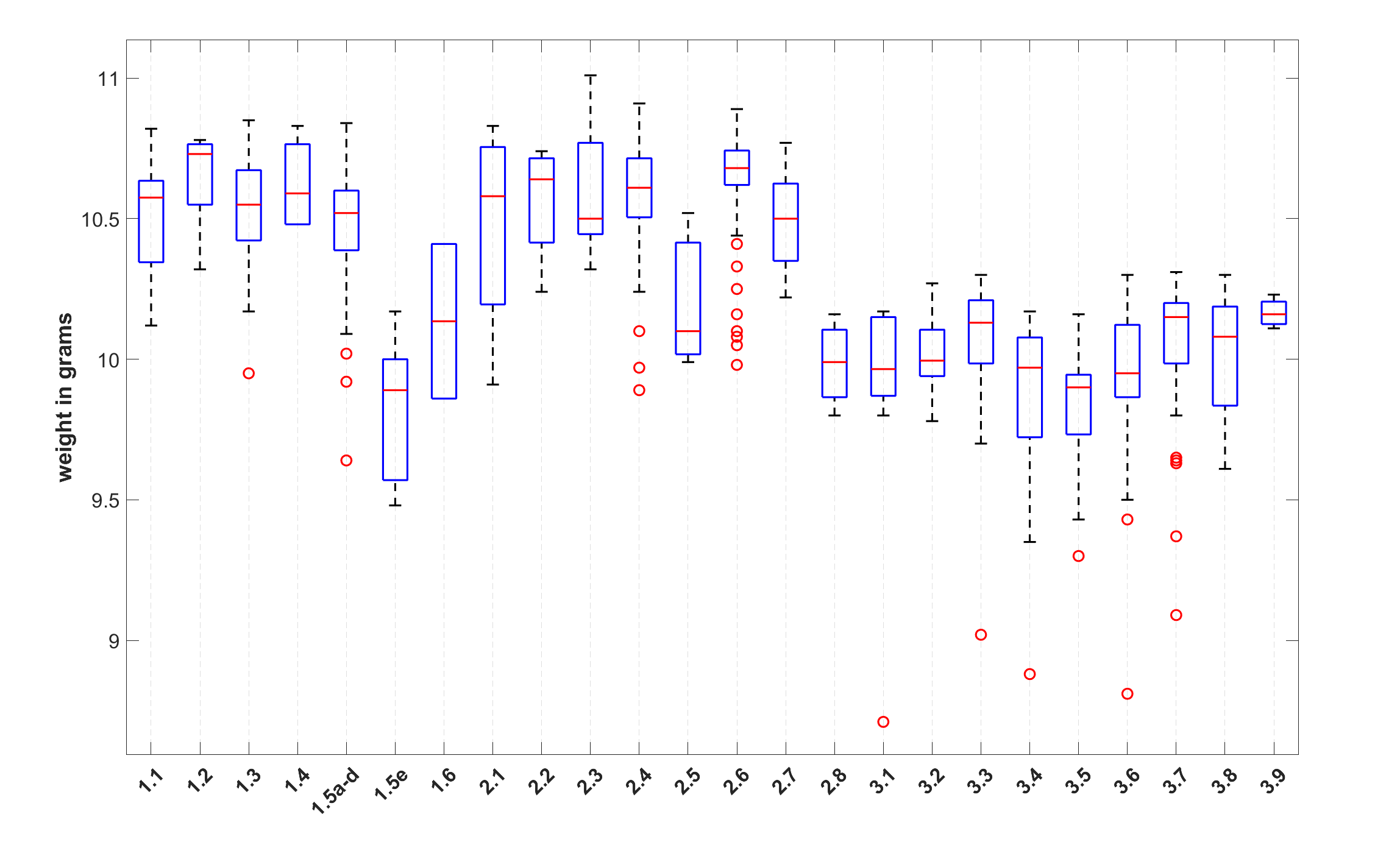
Figure 1: Box plots of individual coin types

Type	Count	Mean	Median	Std. Dev.	IQR
1.1	26	10.51	10.57	0.20	0.22
1.2	7	10.64	10.73	0.17	0.21
1.3	43	10.55	10.55	0.19	0.26
1.4	4	10.62	10.59	0.17	0.29
1.5a-d	46	10.47	10.52	0.23	0.22
1.5e	14	9.85	9.89	0.24	0.43
1.6	2	10.13	10.13	0.39	0.55
2.1	4	10.47	10.58	0.40	0.56
2.2	5	10.56	10.59	0.20	0.23
2.3	8	10.59	10.50	0.23	0.33
2.4	42	10.52	10.61	0.29	0.25
2.5	3	10.20	10.10	0.28	0.40
2.6	169	10.66	10.68	0.15	0.12
2.7	13	10.51	10.52	0.18	0.30
2.8	4	9.98	9.99	0.16	0.24
3.1	15	9.90	9.96	0.35	0.27
3.2	12	10.02	9.99	0.14	0.17
3.3	12	9.91	10.11	0.45	0.41
3.4	50	9.88	9.96	0.26	0.35
3.5	18	9.84	9.91	0.20	0.18
3.6	29	9.93	9.95	0.29	0.27
3.7	44	10.05	10.14	0.25	0.21
3.8	11	10.00	10.08	0.23	0.35
3.9	4	10.16	10.16	0.05	0.08

Table 2: Basic descriptive statistics of individual coin types

As shown in Figure 1 and Table 2, similar to Type 1.5e in Group 1, Type 2.8 in Group 2 is distinguished by its lower weight. The mean and median weights of these two types correspond to those of Group 3. Types 1.6 and 2.5 also seem to be somewhat close in weight to Group 3, but since their lower weight is not so significant, it cannot be ruled out that this is merely a random deviation due to the small number of specimens in the analysed corpus (2 specimens for Type 1.6 and 3 specimens for Type 2.5).

Based on these observations, we can adjust the catalogue groups of coins in terms of weight standard as follows:

Group A:	coins of Group 1 except Type 1.5e;
Group B:	coins of Group 2 except Type 2.8;
Group C:	coins of Group 3 with Types 1.5e and 2.8.

Table 3 shows the descriptive statistics of Groups A, B and C. Figures 2–4 visualise the weight distributions of these groups: box plots, relative frequency histograms (the bars represent the relative frequencies of observations ranging from 8.70 to 11.10 g in increments of 0.10 g) with the continuous curves representing approximations of the data by the Weibull distribution2, and cumulative distributions.

Statistics	Group A	Group B	Group C
Number of coins:	128	244	213
Mean:	10.51	10.62	9.94
Standard deviation:	0.22	0.20	0.27
Interquartile range:	0.25	0.17	0.30
Skewness:	-1.17	-2.12	-1.74
Kurtosis:	4.87	9.47	7.15
Minimum:	9.64	9.42	8.71
25th percentile:	10.41	10.57	9.85
Median:	10.55	10.66	9.99
75th percentile:	10.66	10.74	10.15
Maximum:	10.85	11.01	10.31

Table 3: Descriptive statistics of adjusted coin groups

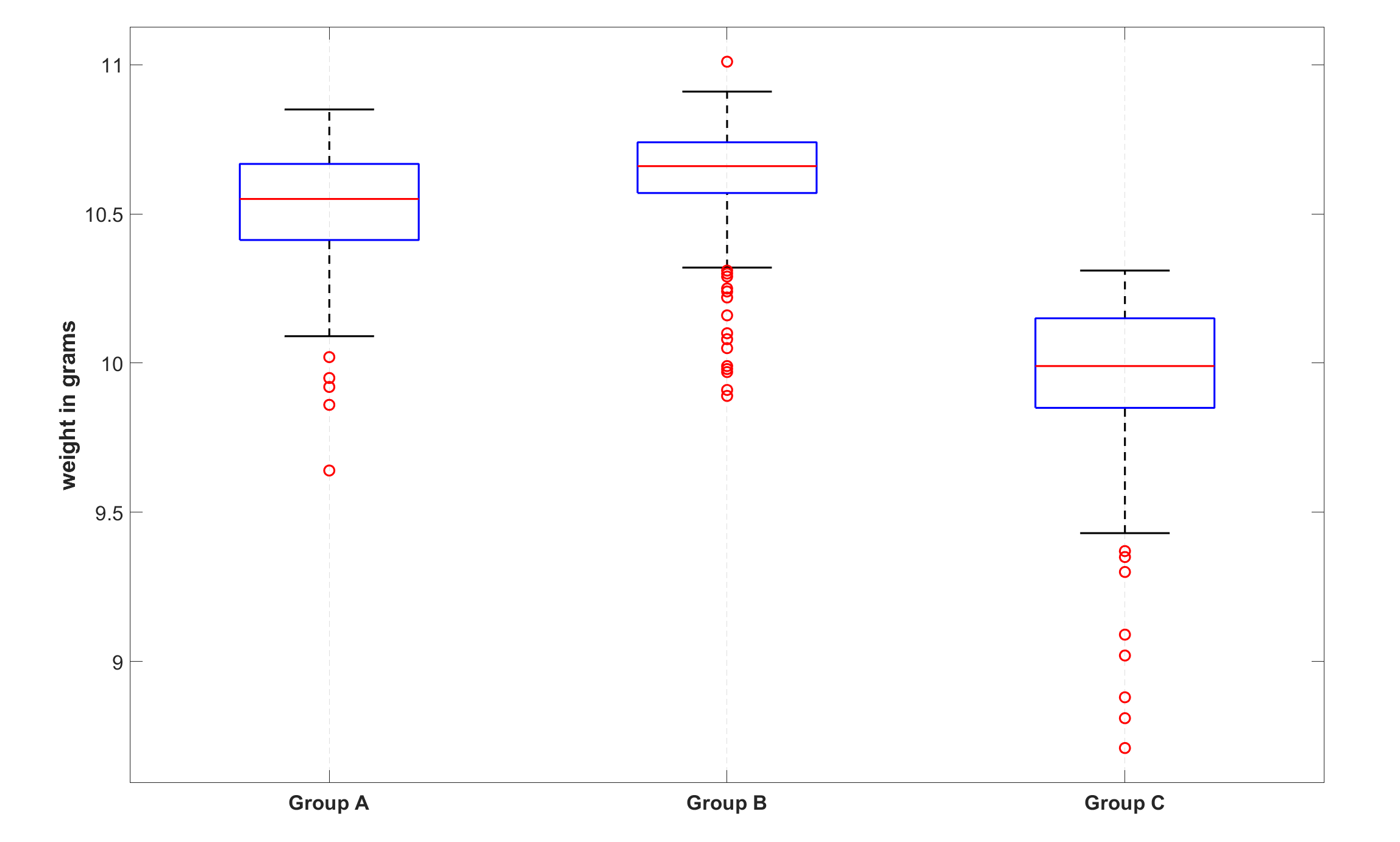
Figure 2: Box plots

Figure 3: Relative frequency histograms

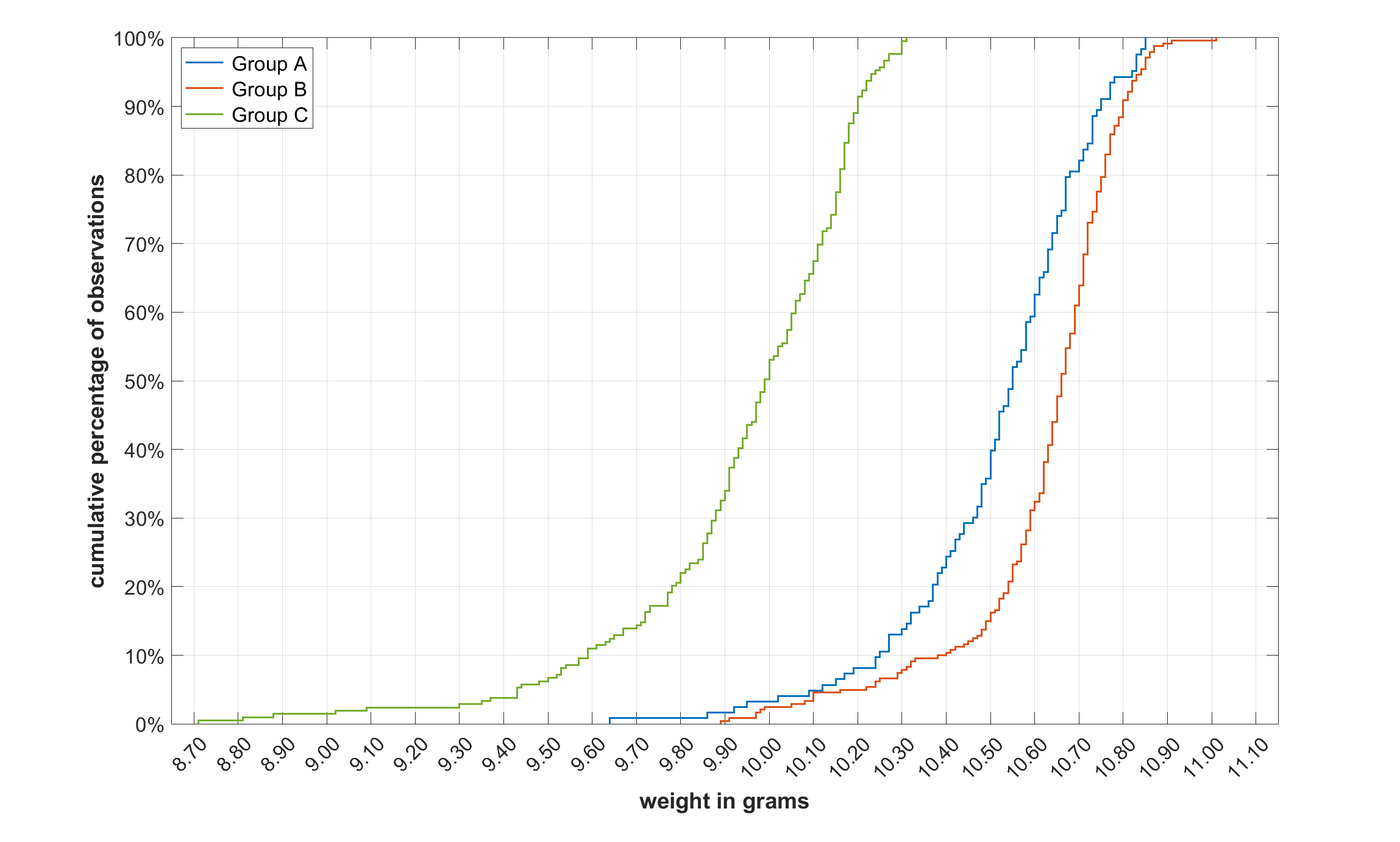
Figure 4: Cumulative distributions

The two-sample Kolmogorov-Smirnov tests reject the hypothesis that the weight distributions of Groups A, B and C are equal, with the p-value being less than 0.001 for all three of these paired tests. Given the Bonferroni correction (0.05/3 = 0.0167), we can conclude that the distributions of the weights of Groups A, B, and C are different. As Table 3 and Figures 2–4 show, Group B has the highest average and median weight, followed by Group A and then Group C. This is also confirmed by the one-sided Welch’s t-tests3, which all have p-values less than 0.001, i.e. less than the criterion for Bonferroni correction. The percentile bootstrap method was also used to supplement these results. Table 4 shows the observed sample medians and bootstrap 95% confidence intervals.4 Table 5 shows the difference in sample medians, its bootstrap 95% confidence interval and p-value.5 These results confirm the descending order B–A–C in terms of weight.

	median	95% confidence interval
Group A	10.55	10.51	10.59
Group B	10.66	10.64	10.68
Group C	9.99	9.95	10.04

Table 4: Medians and their confidence intervals

	difference in medians	95% confidence interval		p-value
Group A vs Group C	0.56	0.50	0.61	<0.001
Group B vs Group A	0.11	0.07	0.16	<0.001
Group B vs Group C	0.67	0.62	0.71	<0.001

Table 5: Differences in medians