Summary Analysed coins Analysis

Summary

This analysis examines the weights of fourrées imitating the official staters of Kelenderis and Nagidos. The analysed specimens of fourrées imitating Nagidos staters are mostly heavier than the analysed specimens of fourrées imitating Kelenderis staters: the differences between the mean and median weights of these two groups are 1.15 g and 1.27 g, respectively. This surprising fact is due to Kelenderis fourrées of Types 3 and 4, characterised by a square incuse on the reverse, which are significantly lighter than other fourrées. Perhaps a different production technique was used, or they came from a different unofficial mint from the other fourrées (the low quality of the dies indicates that they came from an unofficial mint).

Analysed coins

Coin catalogue sections:	Kelenderis, Fourrées, Nagidos, Fourrées
Coin corpus datasets:	Kelenderis, Fourrées, Nagidos, Fourrées

The numbers of analysed coins are given in Table 1. Coins whose weight is unknown or unreliable, or that are excessively corroded or damaged, are excluded from the analysis.

Corpus	Number of coins as of 2 November 2025
	Total	Excluded	Analysed
Kelenderis, Fourrées	28	3	25
Nagidos, Fourrées	11	1	10

Table 1: Numbers of analysed coins

Analysis

Descriptive statistics for all fourrées and separately for Kelenderis and Nagidos are presented in Table 2, while box plots1 are shown in Figure 1.

Statistics	All fourrées	Kelenderis	Nagidos
Number of coins:	35	25	10
Mean:	7.74	7.41	8.56
Standard deviation:	1.39	1.50	0.50
Interquartile range:	1.90	2.15	0.69
Skewness:	-0.38	0.11	-0.64
Kurtosis:	2.21	2.02	2.95
Minimum:	4.87	4.87	7.53
25th percentile:	6.82	6.25	8.26
Median:	7.92	7.33	8.60
75th percentile:	8.72	8.40	8.95
Maximum:	9.90	9.90	9.29

Table 2: Descriptive statistics of coin groups

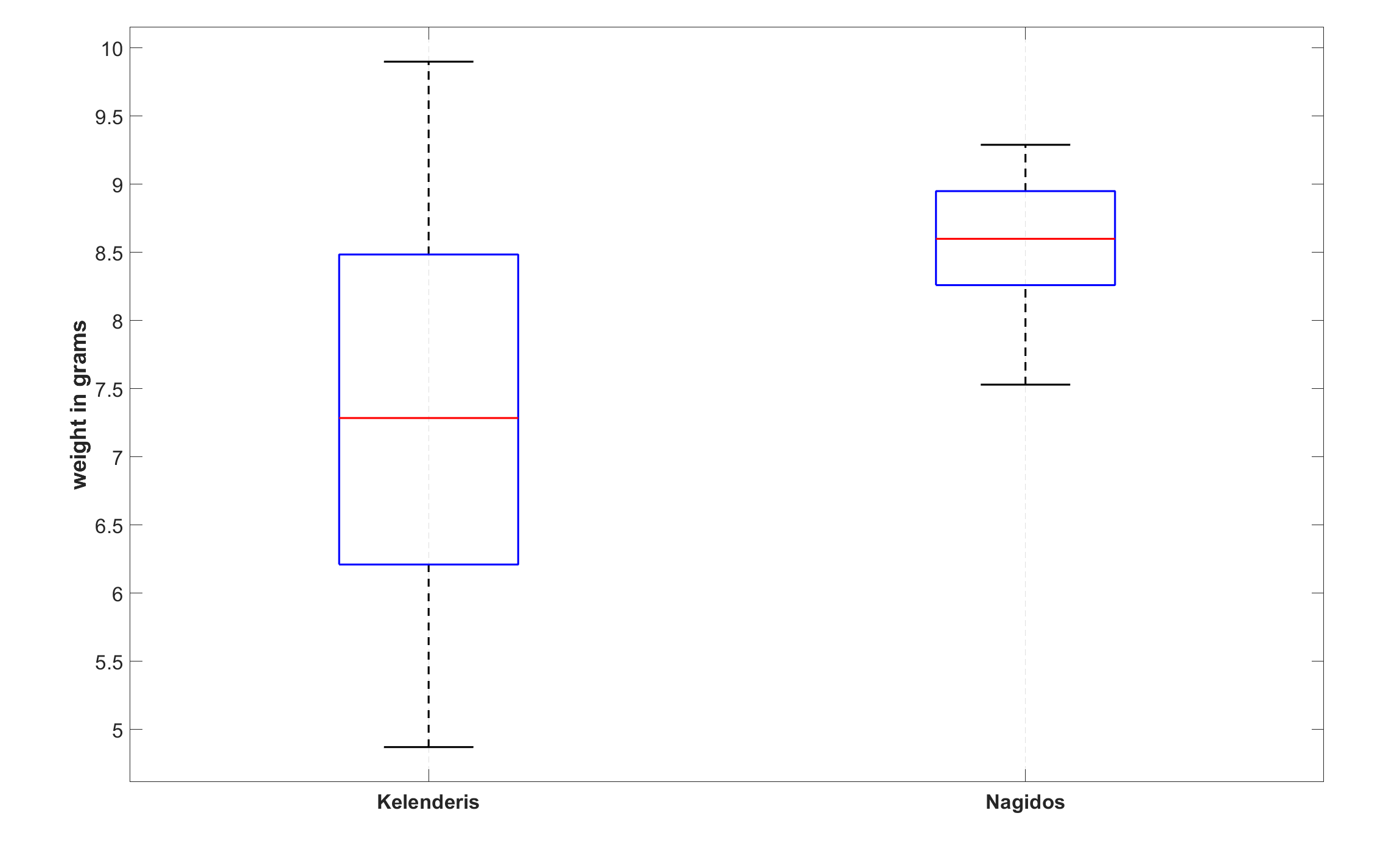
Figure 1: Box plots of the Kelenderis and Nagidos fourrées

These results suggest that fourrées imitating Nagidos staters were usually heavier than fourrées imitating Kelenderis staters. Indeed, the two-sample Kolmogorov-Smirnov test rejects the hypothesis that the weight distributions of the Kelenderis and Nagidos fourrées are equal (p-value of 0.004). Similarly, the one-sided Welch’s t-test2 rejects the null hypothesis that the mean weights of both groups are equal in favour of the alternative that the mean weight of the Kelenderis fourrées is less than that of the Nagidos fourrées (p-value of 0.001).

A closer look at the corpus of the Kelenderis fourrées, however, shows that most of their lightweight specimens belong to Types 3 and 4, which are characterised by a square incuse on the reverse (for Type 4 it is not certain, but quite likely). Table 3 presents descriptive statistics (Std. Dev. denotes the standard deviation and IQR the interquartile range) and Figure 2 shows box plots when the Kelenderis fourrées are divided into two groups. Types 3 and 4 appear to form a separate group within the Kelenderis fourrées. Perhaps a different production technique was used, or they came from a different unofficial mint from the other fourrées (the low quality of the dies indicates that they came from an unofficial mint).

Note that Table 3 and Figure 2 indicate that the Kelenderis fourrées other than Types 3 and 4 are slightly heavier than the Nagidos fourrées. However, the low number of observations (7 Kelenderis fourrées other than Types 3 and 4, and 10 Nagidos fourrées) does not allow us to draw any conclusions. As expected, the one-sided Welch’s t-test does not reject the null hypothesis that the mean weights of both groups are equal (p-value of 0.090).

Type	Count	Mean	Median	Std. Dev.	IQR
Kelenderis, Types 3 and 4	18	6.74	6.86	1.07	1.99
Kelenderis, other types	7	9.14	9.50	0.96	0.92
Nagidos	10	8.56	8.60	0.50	0.69

Table 3: Descriptive statistics with the Kelenderis fourrées divided into two groups

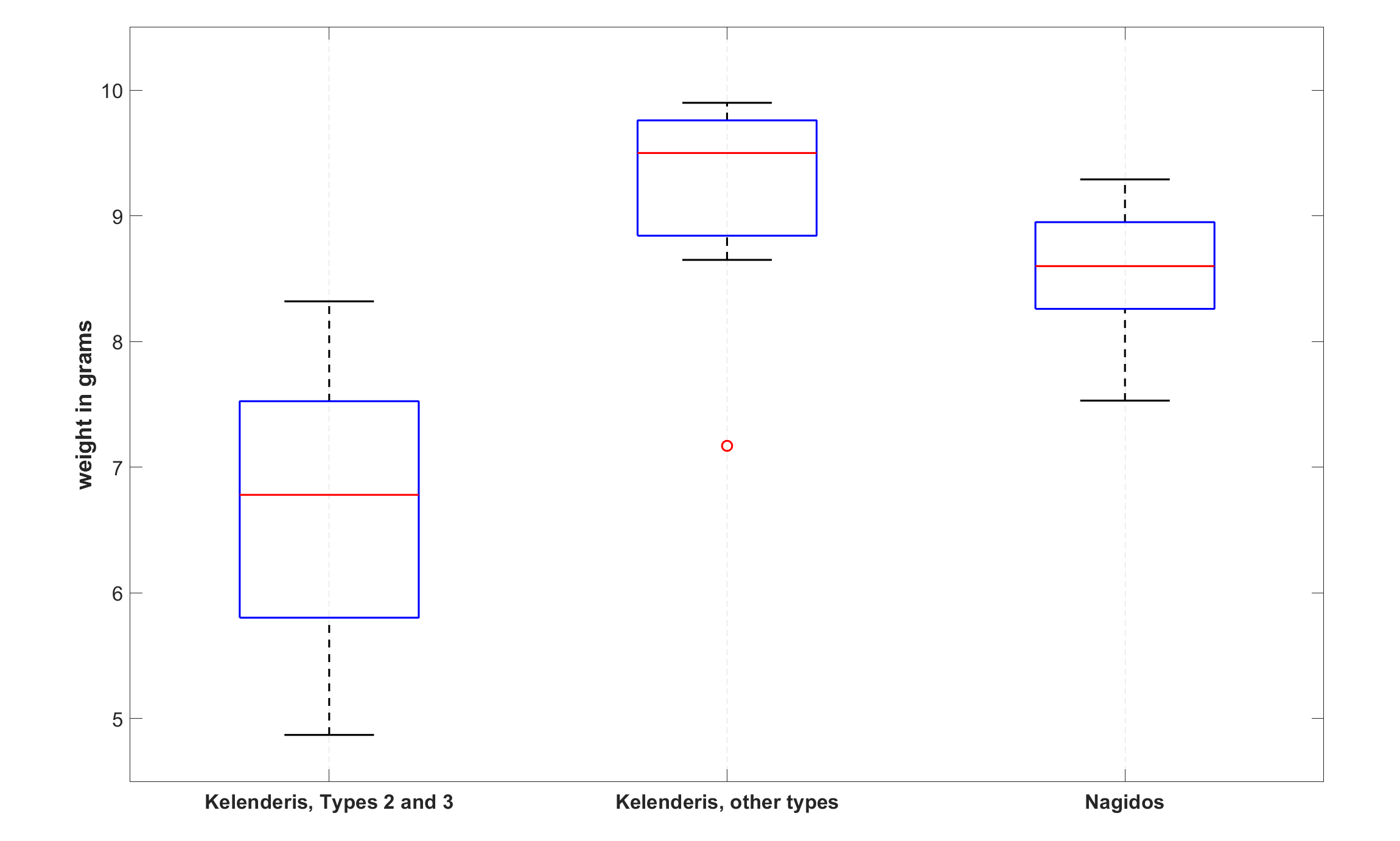
Figure 2: Box plots with the Kelenderis fourrées divided into two groups

The following two charts visualise the weight distributions of fourrées of these two cities in greater detail. Figure 3 presents relative frequency histograms (the bars represent the relative frequencies of observations ranging from 4.50 to 10.00 g in increments of 0.50 g), with the continuous curves representing approximations of the data by the Weibull distribution3 based on maximum likelihood estimates. Cumulative distributions are shown in Figure 4. In both charts, Types 3 and 4 of the Kelenderis fourrées are distinguished by a lighter blue colour.

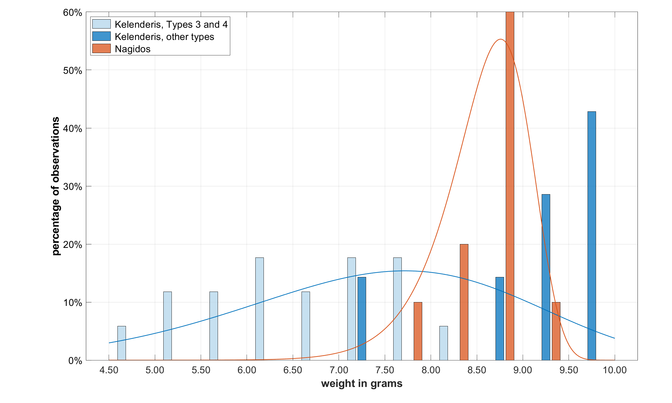
Figure 3: Relative frequency histograms of the Kelenderis and Nagidos fourrées

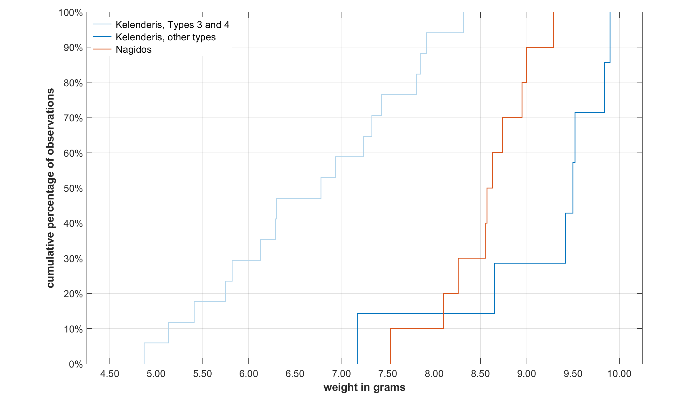
Figure 4: Cumulative distributions of the Kelenderis and Nagidos fourrées